How Mathematics Finds the Optimal Route

Introduction
Have you ever been in an unfamiliar place and need to get somewhere? The solution, inevitably, is to go on Google Maps and mindlessly follow its route. But have you ever wondered how it finds the fastest way so quickly? After all, there are millions of possible routes that you could take to reach the destination. So how can a computer find the optimal path without testing every potential journey?
To capture the essence of the idea, we must map the roads as a graph where roads are edges and the junctions are nodes. Each road has a weight, which could be time or distance. The shortest total journey time will be the one where the total weight from A to F is the smallest. Use the diagram below to find the quickest route.
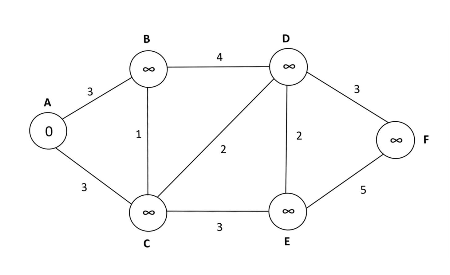
Simple addition tells us that the path: A — C — D — F is the fastest, yielding a total weight of 8. This same concept can be applied to actual roads with sophisticated algorithms. What you have just done by finding the shortest path is a simplified version of what applications like Google Maps do.
Dijkstra’s Algorithm
Dijkstra’s algorithm is one such way of calculating the shortest distance between 2 places. The essential method is as follows:
1. Start at A (the source node)
2. Give A a distance of 0 as the distance from A to itself is 0
3. The distances of all remaining nodes (B, C, D, E and F) are set to infinity since they have not been reached yet
4. Look at the neighbouring nodes and record the shortest distance to each one
5. Move to the unvisited node with the smallest distance
6. Repeat until reaching the destination (F)
To put this in practice, the distance to node B is 0 + 3 = 3 and the distance to C is also 3. Since these distances are smaller than the previous value (∞), they are updated. Dijkstra’s algorithm then goes to the unvisited node with the smallest distance. In this case, B and C both have a distance of 3 so the algorithm can choose either one. Let us say that it chooses B. It then looks at the unvisited neighbours of B. The distance of C through B is 3 + 1 = 4. However, this is greater than the current distance of C so the distance is not updated. The distance of D through B is 3 + 4 = 7. 7 is less than ∞ so the distance is updated. The next unvisited node that is closest to the source node (A) is C. Dijkstra’s algorithm then inspects C’s unvisited neighbours. The distance to D through C is 3 + 2 = 5, which is smaller than the previous distance (7). Therefore, the distance to D is updated to 5. The path length to E is 3 + 3 = 6, which is less than ∞. The distance is adjusted accordingly. The nearest unvisited node is D (distance of 5). The only unvisited neighbours from D are E and F; the resulting distance to E is 5 + 2 = 7, which is greater than its current distance of 6. F has a total distance of 5 + 3 = 8. 8 is less than ∞ so the distance is recalculated. Finally, the last 2 unvisited nodes from E are D and F. The distance to D via E is 8, which is more than the tentative distance, so it stays at 5. The distance to F is 6 + 5 = 11. Because 11 > 8 the total distance to F from A is not updated. Now all the nodes have been visited. The quickest route to F is therefore A — C — D — F, as calculated before. The completed diagram can be found below.
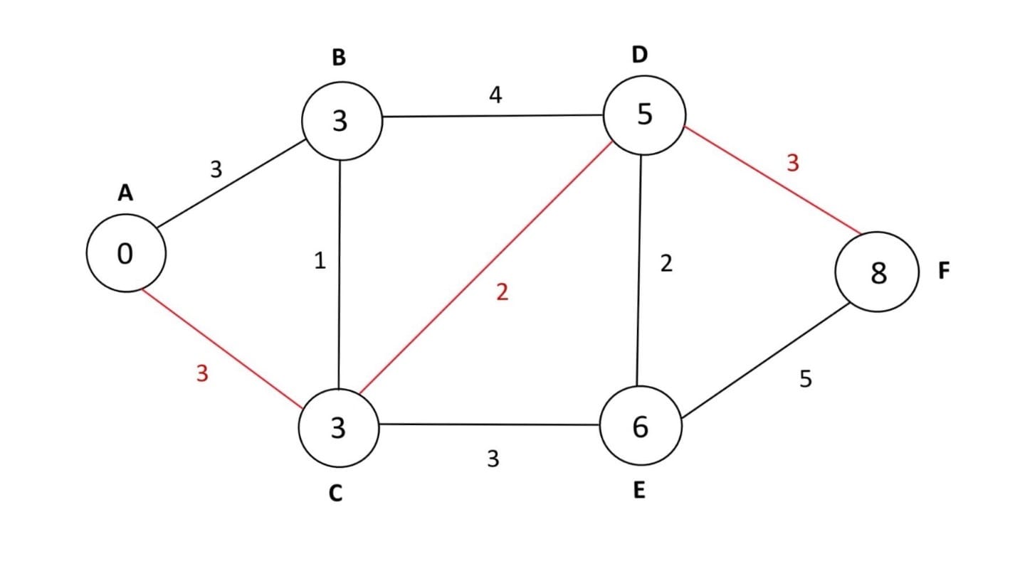
There are other algorithms to find the fastest route, which improve upon Dijkstra’s algorithm in some respects. Imagine you are in a dark room and want to find the way out. Using Dijkstra’s algorithm is like exploring outwards from the starting point in an ever-expanding circle. While you would be guaranteed to find the shortest path, it would waste a lot of time, exploring places that are nowhere near the exit. On the other hand, in the same dark room, utilising the A* algorithm would be like having a compass that points towards the exit – instead of exploring blindly, you would use the compass to guide you in the right direction, saving you valuable time.
A* Algorithm
A* uses an estimate of how far each point is from the destination, called a ‘heuristic’. For example, if you are travelling from Windsor to London, the straight-line distance between your current position and London gives a rough estimate of how much of the journey is left. A* combines 2 quantities and can be expressed as the equation below:
f(n) = g(n) + h(n)
g(n) is the actual time/distance from the start to the junction ‘n’ being considered
h(n) is how much of the journey is left after junction ‘n’
f(n) is the total estimated journey distance/time from the start to the desired destination
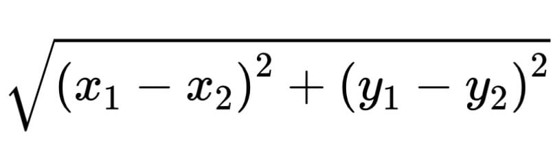
The algorithm prioritises routes with the smallest value of f(n). For example, if a particular junction takes 6 minutes to reach and is estimated to have 4 minutes left, while another junction takes 8 minutes to reach, with only another minute left, A* would inspect the second junction first as the total estimated time – f(n) – is shorter. This significantly reduces the number of different paths that need to be examined, hereby calculating the journey faster. Crucially, heuristic must not overestimate the remaining distance/time if it wants to be able to find the optimal path because if it is overestimated, the algorithm may accidentally rule out the fastest path. This is why straight-line distance is useful as it is the shortest possible distance between the 2 points. It is measured with the Euclidean distance formula:
Differences between Dijkstra and A*
A key difference between Dijkstra’s algorithm and A* is that Dijkstra decides which point to explore solely on g(n) — how far or how long have you already travelled? So, if A — B is 3km and A — C is 5km, it will investigate A — B first as g(n) is less. However, say the straight-line distance C — D is 2km and B — D is 6km, A* will inspect the route through C first, even though it is further from the start. It is important to note that while edge weights can be either distance or time, the end goal is to minimise time. So, a shorter path might not necessarily be faster than another with a longer distance. Applications like Google Maps have to use your real-time speed along with the speed of others around you. They also have to adapt to ever changing traffic.

The Problem of Predicting Traffic
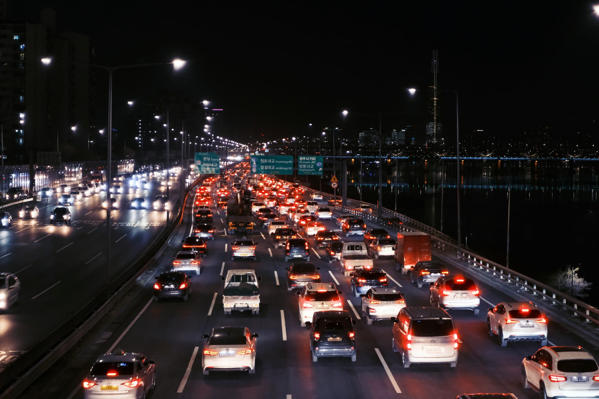
The weights, therefore, cannot be fixed, as they change with traffic conditions. A road could take 10 minutes to go through at 07.30 and take 45 minutes at 8.30. Because of this, the route is constantly adjusted and even changes while a journey is still in progress. To calculate the traffic, Google uses historical data about how fast cars usually go on a certain length of road at a certain time, along with data from smartphones and sensors, telling Google how fast the cars are going.
When you go on to Google Maps with your location on, your phone anonymously sends information to Google, telling them how fast you are going. They can then use this information from all the cars on the road who are using Google Maps to see how fast the everyone is travelling on average. So, if lots of people in front of you slow down, Google can tell that there is some sort of traffic jam, meaning that it diverts your route. It also uses patterns such as rush hours to be able to predict where, how long and when a jam will happen before it even happens. It uses a machine learning system called Graph Neural Networks to generate a remarkably reliable prediction. Moreover, in 2013, Google acquired Waze, where people can report if there has been an accident or a slowdown, helping people around them be aware of which route they should take. It also adds a more human aspect to route planning, rather than putting all trust into a machine. This all culminates in an impressive accuracy rate, of over 97%.
When Everyone Takes the Best Route
There is, however, another complication. Imagine there are 1000 drivers who want to get from A to B. There is a motorway which takes 20 minutes and a smaller road that takes 25 minutes. Nearly all the drivers would take the motorway as it is quicker. Since there are more and more cars going on the motorway, slowly traffic increases and so Google Maps updates the times: the motorway takes 30 minutes while the smaller road stays at 25 minutes. Suddenly, all incoming drivers faced with the choice would now pick the smaller road, but then that will get congested as well. The decision of each drivers affects the journey times for everyone else. This concept introduces the counterintuitive Braess’ Paradox, which postulates that adding a new road to a road network could increase the travel time of each driver. For example, let’s say there are 2 routes around a lake, A and B, which take the same amount of time — 10 minutes to get around it to destination X. Suddenly, a bridge is built across the lake, acting as a shortcut straight from the start to X, and it should take only 2 minutes to get across. Now everyone will take the bridge because it is the fastest in theory. However, as everyone will now take the bridge, the total journey time for each driver actually increases to 15 minutes, meaning that it would have been better if the only 2 routes were A and B. Also, nobody would want to go back to going through either route A or route B as it would psychologically mean committing to an extra 8 minutes of travel time, rather than taking the ‘faster’ shortcut.


Hence, the best route for one driver is often different from the most optimal route for the overall network. In the future, applications like Google Maps may have to consider not only the best route for the individual, but also the optimisation of the network as a whole. They could potentially do this with network aware routing - giving different people alternative routes with similar travel times, preventing traffic on some particularly congested roads. A study was conducted by Google this year on this topic and was found to have improved traffic for the overall network.
Conclusion
The next time you use Google Maps, do not just automatically follow that blue line, but instead take a moment to think about the complicated maths that goes behind optimising your journey, from graph theory and algorithms to traffic modelling. Google Maps manages to do all of this for the entire world, continuously solving a problem that is always changing.
Bibliography
Arora, Neha, and Aboudy Kreidieh. "The Power of Collaboration: How We Can Reduce Traffic Congestion." 7 July 2026, research.google/blog/the-power-of-collaboration-how-we-can-reduce-traffic-congestion/.
"Braess' Paradox." brilliant.org/wiki/braess-paradox/.
Brindle, Beth. "How Does Google Maps Predict Traffic?" electronics.howstuffworks.com/how-does-google-maps-predict-traffic.htm.
"Dijkstra's Algorithm." Wikipedia, the Free Encyclopedia, Wikimedia Foundation, Inc, 11 Mar. 2026, en.wikipedia.org/wiki/Dijkstra%27s_algorithm.
Kumar, Rajesh. "The A* Algorithm: A Complete Guide." 7 Nov. 2024, www.datacamp.com/tutorial/a-star-algorithm.
Lange, Oliver, and Luis Perez. "Traffic Prediction with Advanced Graph Neural Networks." Google DeepMind, 3 July 2026, deepmind.google/blog/traffic-prediction-with-advanced-graph-neural-networks/.
Lau, Johann. "Google Maps 101: How AI Helps Predict Traffic and Determine Routes." Google, 3 Sept. 2020, blog.google/products-and-platforms/products/maps/google-maps-101-how-ai-helps-predict-traffic-and-determine-routes/.