Disease as a threat on endangered species
Disease has only accounted for the extinctions of less than 4% of known species since 1500, and only affects around 8% of species now listed as critically endangered, according to National Institute of Health studies. While it lacks a major role in the overall force of extinction for species around
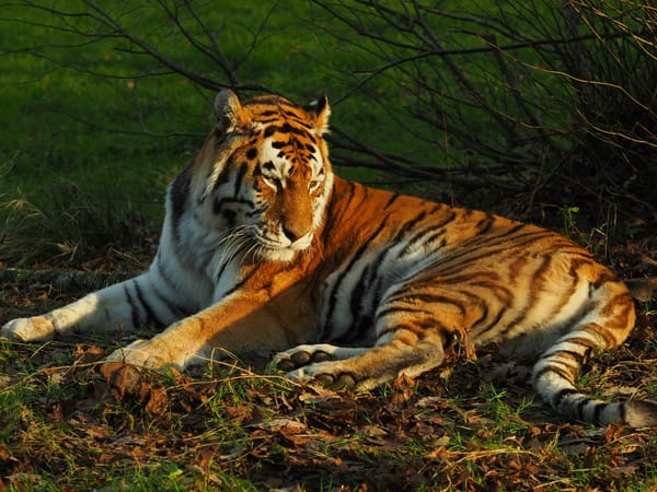
![Image via [Adobe Stock]](/content/images/size/w600/2026/03/IMG_0874.jpeg)